A Neural Network Family Tree

So far, we have just looked at one particular architecture - the Multi-Layer Perceptron. Admittedly, this is probably the most common architecture, and its behavious is well understood. However, there are others and they have their uses in different situations. I have duplicated the following diagram from Lippmann's paper An Introduction to Computing with Neural Nets, which shows a taxonomy (classification) of possible neural network architectures. At the end of each branch, there is a sample architecture in that classification, but I'm sure you will come across others which aren't mentioned in the diagram.

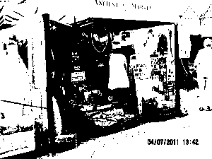
Binary vs. Continuous Input

Single-layer Perceptrons (referred to simply as "Perceptrons" in the diagram above) and Multi-Layer Perceptrons take any input values in a given range. Typically, that range is 0 to 1, but it is possible to train neural networks with wider input ranges (-1 to 1 is another common input range). Although the training methods become less reliable if you expand the range of the possible input values (say to the range 0 to 100), even situations like this can be accommodated by prescaling the inputs into a form suitable for the network (see the section on Coding the Inputs).

However, there are some neural network architectures that can only cope with binary inputs, i.e. inputs that two discrete values with nothing in between. This includes the case where the inputs can be cast in the form of 1s and 0s (obviously), but also the networks such as the Hopfield net which has inputs that are either 1 or -1.

Although such networks cannot inherently cope with "shades of grey", they do still have their uses. Image input, for instance, can be hard-limited so that each pixel in the image is either black or white, as shown with the following photograph. Although this involves the loss of a great deal of detail, the image is still recognisable to human eyes, and, often getting rid of the detail can improve neural network performance by decreasing the amount of signal "noise" in the image.

    

Such a simple hard-limiting algorithm allows a neural network based on the WISARD architecture to act as an intruder detector for a CCTV system, for instance. Alternatively, shades of grey and indeed colours can be coded into pure binary format using several bits of data. This does mean increasing the number of inputs to the network but does allow the use of these binary networks in situations where the detail of the image is important.

Supervised vs. Unsupervised

One problem that people tend to raise when I discuss neural networks is "Who is going to teach all these data-hungry networks?" The answer may be "Themselves". That is certainly the case for unsupervised networks.

Multi-layer perceptrons are a supervised architecture, which means that they have to be given the training patterns, each clearly labelled with what it's supposed to be (i.e. the desired output is given along with each training pattern). However, with unsupervised architectures, such as the Carpenter-Grossberg Network or the Kohonen Net, the various training patterns are each presented to the network unlabelled, and the network decides for itself how the pattern should be classified. You might ask how this is possible, since the network doesn't know what it's supposed to be recognising, but the network would automatically sort patterns into groups depending on their similarity. For example, a Kohonen net used for speech recognition might produce one set of outputs for an input pattern "cat" and a different one for "dog" (since they sound sufficiently different that they wouldn't be confused). If it received another, slightly different, pronounciation of "cat" (possibly in a different regional accent), that pronounciation would be categorised along with the previous "cat" provided it was sufficiently close to in terms of the inputs provided to the network. If it was very different (perhaps a broad Glaswegian pronounciation of "cat" as opposed to a West Country pronounciation), the network might (wrongly) classify it as a completely new word.

Autoassociative Networks

So far the networks that we have seen have taken a particular input pattern and produced a (different) output pattern from it. However, several of the networks that appear on the family tree above are autoassociative, meaning that the output pattern that they produce is the same as the input. This may sound a bit stupid, and, the way I've phrased it, it is, so I'd better explain.

Autoassociative networks are trained with certain training patterns, so that if they are presented with versions of those patterns that are in some way "faulty" (e.g. parts of the pattern are missing or a great deal of signal "noise" is added to the image), they can recreate the original patterns. The following example is also duplicated from Lippmann's paper (a marvellous introduction to Neural Networks, incidentally - well worth a read!), in which an associative network has been trained on the following series of patterns:

Generally speaking, autoassociative networks are iterative, which means that they loop round and round, gradually getting closer and closer to one of the training patterns. Here the Lippmann network has been presented with some random pattern, and it gradually loops round and round getting closer to (in this case), the "3" pattern. However, you will notice that it doesn't recreate it perfectly (but good enough).